The centrality of experimental design, part 1

At C4DM, we are organising a seminar/tutorial series about statistics aimed at graduate students (and ourselves). We will address persistent and fundamental questions we all have when we go about collecting and/or analysing data. Which statistical test should I use and why? How many subjects/observations do I need? Can I get away with 20? What can I validly conclude? There is a massive literature about statistics (it is one of the greatest achievements of the 20th century), but it will remain opaque as long as its fundamentals are absent in the training of researchers.

My tutorial on Dec. 15 will focus on why experimental design is central to answering these common questions. Just plugging one’s data into statistical packages and comparing p-values before considering the data collection is as senseless as shelling a clam after eating it. To demonstrate this, consider the following scenario:

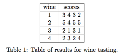
As the local data science experts, we are contacted by a local chapter of oenophiles eager to have their data analysed in order to create an official ranking of local wines. They send us the table of results below with the description: “Four professional judges tasted four wines and scored each on a scale 1-5 (poor to excellent). Which wine is the best, and which is the worst, according to these judges? kthxbai!”

Let’s begin with some basic analysis.

We start by computing some descriptive statistics of each wine from Table 1: mean , (unbiased) standard deviation , and standard error of the mean (SEM) . These are shown in Table 2.

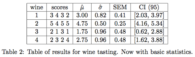
Wine 2 could have the highest mean score, wine 3 could have the lowest, and wines 1 and 4 are somewhere in the middle. Are these significant? Assuming each mean is distributed Normal, but with unknown variance, we compute its 95% confidence interval (CI, 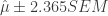, using t-distribution with 3 degrees of freedom). The figure below shows these intervals for each wine.

We see from this that we might conclude at a significance level that the mean score of wine 2 is significantly different from all the others. Performing ANOVA on all the scores produces a p-value of 0.0021, which motivates rejecting the null hypothesis that there are no differences between the scores. Table 3 shows the results of pairwise comparisons on the scores of each pair of wines using ANOVA. This also confirms wine 2 appears to be significantly different from the other three. It is a clear winner!

We cannot conclude, however, that the mean scores of the other wines are significantly different from each other. Our estimated mean scores of wines 1 and 4 are higher than that of wine 3, but this could be due to chance. There are no clear losers, in other words.

A serious question to consider is how our analysis is impacted by the fact that the measurements are restricted to be integers in [1, 5]. No doubt, we could apply a variety of different tests, depending on the different ways we define “best” and “worst”; but doing so is jumping the gun because we haven’t considered the most important question first: What can we validly conclude from the results in Table 1?

I will show that in fact nothing can be concluded about these wines, no matter the scores in Table 1, because (SPOILER ALERT) the experimental design that led to its creation is “messed up.” In more general terms, I will show how the meaningful analysis of this data actually turns on the way the data was collected in the first place — the experimental design. This will demonstrate how “which statistical test to use and why” can be sensibly answered only after considering the experimental design.